Welcome to Transplanet
The synopsis of IPIM ionosphere model (Marchaudon and Blelly, 2015) is presented in figure 1. This model is a legacy of TRANSCAR and TRANSMARS family model (Blelly et al., 1995, Diloy et al., 1996, Blelly et al., 2005) with substantial improvements, the first being that the transport equations for the ionized species are based on a 16 moment approximation (Blelly and Schunk, 1993). The model is basically a one dimensional model, which has been built in a modular way, leading to a core model that is independent from the planet. This core model corresponds to the part delimited by the red line in figure 1. In order to be able to run, it requires some inputs, which are related to the characteristics of the planet.
First of all, the planet is determined by its orbitography and a potential magnetic field that may constrain the geometry; this dependecy is represented by the two green boxes in figure 1. Without magnetic field, the grid used in the model is a vertical grid. But if a magnetic field is present, the grid used for the model is a field aligned grid, which can be an interhemispheric grid.
The other planet-dependent input is the atmosphere (blue box in figure 1) which determines the neutral species that can be considered in the model. The neutral atmosphere is accessible either through an empirical model or a specific profile, which must provide the neutral temperature and the different concentration profiles, and if possible the neutral wind. The interface allows for choosing the neutral components which will accounted for in the run. The neutral species being defined, the core model determines which collisional processes should be retained and thus, the code chooses the chemical reactions, the collision frequencies and the ionization cross sections which are necessary for the model to run (pink boxes in figure 1).
The last inputs required are related to the Sun conditions and correspond to the solar flux which provides the primary production of the ions, and the solar wind couplings with the planetary environment (yellow boxes in figure 1). The external drivers (violet box in figure 1) resulting from these couplings are specific to each planet. In the case of Earth, due to the magnetosphere, the magnetic activity, the precipitation and electrodynamics patterns will characterize these couplings. In the case of Mars, the direct inputs of electrons from the solar wind will characterize these couplings.
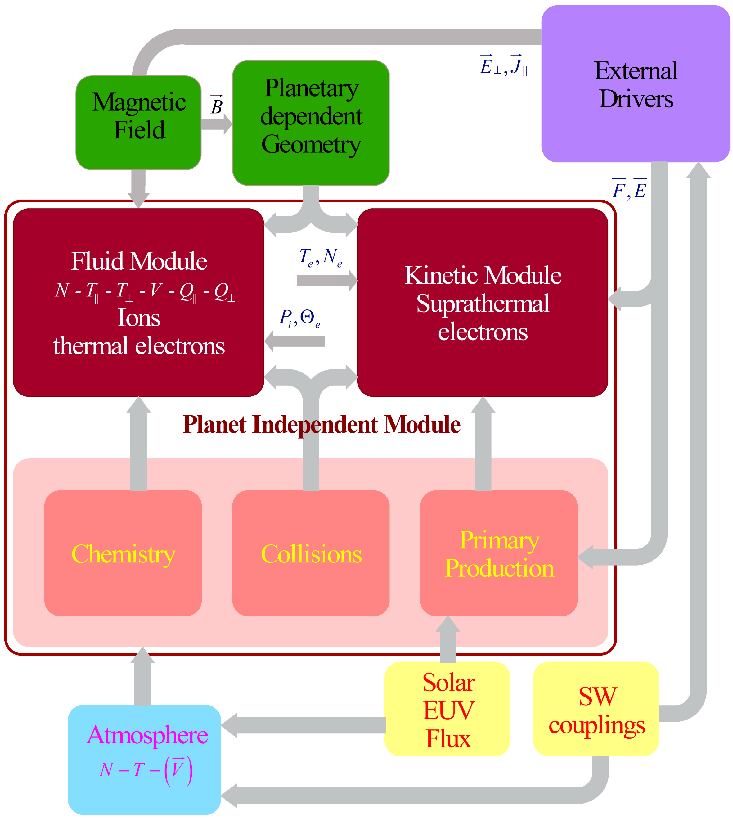
Once all the inputs are defined, the core model can solve for the 1D dynamics of the ionosphere, with the hypothesis that all the vectors are reduced to their projection along the direction solved: vertical if no magnetic field, and field aligned if a magnetic field is present.
This core model is based on two modules which separate the plasma between thermal and suprathermal contributions. The thermal plasma is composed of different ions chosen in the interface and the thermal electrons, and is treated through the fluid module. For every ion considered, this module solves the time-dependent transport equations (field aligned or vertical) of the density, the velocity, the temperature (parallel and perpendicular if a magnetic is present) and the heat flux (components related to the parallel and perpendicular temperature). This module accounts for the chemistry and the collisions between the ions and the neutrals.
The suprathermal electrons are obtained from the kinetic module which solves the steady state transport equation of the distribution function of this population. This module accounts for the collisions on the neutrals and excitation and ionization of these species either by electron impact or solar radiation illumination.
Fluid and kinetic modules are coupled so that, the kinetic module provides the total production rates of the ions resulting from the primary production stemmed from the photoionization and the secondary production stemmed from the suprathermal electron impact on the neutrals, as well as the thermal electron heating due the interaction between the suprathermal and thermal electrons (provided by the fluid module).
Solar Flux
One of the main inputs to the model is the EUV solar flux (first yellow box in the flow chart) responsible for atmosphere’s photoionization. In the present version, we use three different solar flux empirical models.
Hinteregger reference spectrum (Hinteregger et al., 1981)
This model provides a solar flux on 22 wavelength intervals (continuum) and 17 lines between 1.9 nm and 103 nm. It is based on two references fluxes, one for maximum solar condition (F10.7 = 243) and one for minimum solar condition (F10.7 = 68) and the dependency on the solar activity is obtained through weighted linear function of F10.7.
EUV Flux Model for Aeronomic Calculations (Richards et al., 1994)
EUVAC model uses different reference spectra with the same wavelength resolution as before. The dependency on F10.7 is basically the same, but the weighted functions differs.
Flare Irradiance Spectral Model (Chamberlin et al., 2007)
FISM model is based on TIMED and UARS satellite measurements and is provided between 0.1 nm and 190 nm with a resolution of 1 nm. The solar flux is avalaible on a daily basis since 1947.
All these solar fluxes are given at L1 (Earth’s distance) and are re-scaled to the position of the considered planet.
Orbitography
Part of the planetary dependent geometry (green box) is constrained by the rotation of the planet and its position along the orbit around the Sun, which defined the relative position of the numerical grid with respect to the planet and sun-planet direction. In order to ease comparisons with space missions, we use Spice kernels as provided by Navigation and Ancillary Information Facility NAIF developed by NASA (Acton, 1996) to define the planet frame and orbitography.
Planet dependent inputs
As mentioned above, the geometry is planetary-dependent (first green box in the flow chart): along magnetic field lines for magnetized planets and radial otherwise. In case of magnetized planets, magnetic field empirical models (second green box in the flow chart) are used as inputs, taking into account only the first eight spherical harmonics coefficients allowing for a dipolar eccentric analytical description of the magnetic field.
The external drivers (light purple box in the flow chart) are optional inputs which cover: convection electric field, field-aligned currents, magnetospheric particle precipitation in the case of a magnetized planet or solar wind particles direct entry otherwise. Currently, these inputs have only been set up for the Earth’s case and are given by empirical models.
Atmosphere and electrodynamics inputs are generally driven by the degree of solar wind coupling (second yellow box in the flow chart) which is characterized by magnetic activity in the terrestrial case.
Earth
Magnetic field
The magnetic field is derived from IGRF-12 (Thébaut et al., 2015). Using the eight first coefficients of IGRF model, we compute the characteristics of the equivalent eccentric tilted dipole, which is used to define the magnetic field line geometry.
Atmosphere
The neutral atmosphere model used is NRLMSISE-00 (Picone et al., 2002) for density and temperature and HWM-93 (Hedin et al., 1996) for winds.
Electrodynamics
Different convection models can be used in the code and may address convection patterns either in the magnetic equatorial plane or in the auroral region. For historical reasons, the basic convection model used are auroral region Senior et al. (1990) model and Schulz (2011) magnetospheric convection model. The electron precipitation model is taken from Hardy et al. (1987).
Atmosphere and electrodynamics inputs are driven by magnetic activity obtained from the Ap magnetic index (Bartels, 1938).
Mars
Atmosphere
The Neutral atmosphere is taken from the Mars Climate Database MCD (Forget et al., 1999; Millour et al., 2015), which provides density, temperature and volocities for the different neutral species under different solar conditions.
Jupiter
Magnetic field
The magnetic field is given by the VIPAL’s model (Hess et al., 2011) from which, similarly to the Earth, we use the eight first coefficients to derive the equivalent eccentric tilted dipole.
Atmosphere
The atmosphere is provided through a single profile which is derived from the data obtained during the descent of the Galileo Probe (Seiff et al. 1998).
Outputs of the model
The first outputs of the models are linked to the geometry of the planet. Each grid point is defined by:
- the altitude (alt),
- the curvilinear abscissa (curv),
- the planetocentric latitude, longitude and solar local time (latgeo, longeo, and stl),
- the solar zenithal angle (kiangle),
- the surface and volume of the cell (surface and volume).
These elements are analytically computed either vertically in a spherical frame for non-magnetized planets or along dipolar magnetic field line for magnetized planets.
In case of magnetized planets, other sets of parameters linked to the magnetic field are also defined at each grid point:
- the dip angle between the magnetic field direction and the local horizontal plane (dip),
- the magnetic latitude, longitude, local time and the planetocentric altitude in the eccentric magnetic dipole frame (latmag, lonmag, tmag and Rmag),
- the magnitude of the local magnetic field (Bmag).
The main outputs of the model depending on time, are the moments of the transport equations solved at each grid point and for each charged species α, ions as selected by the user, thermal and suprathermal electrons:
- density (nα),
- radial velocity or field-aligned velocity in case of magnetic field (uα),
- average temperature (Tα) or parallel and perpendicular component of the temperature (T∥α et T⊥α) in case of magnetic field,
- average radial component of the heat flow (qα) or field-aligned components of the heat flow for parallel and perpendicular energy (q∥α and q⊥α) in case of magnetic field.
In addition, the ion production rates (Pα) and the thermal electron heating rate (Heat) at each grid point are also provided.
Finally, the main parameters of the neutral atmosphere are also given at each grid point:
- density (Nn) for each neutral species
- neutral temperature (Tn)
- wind components in geographic frame (Un=0, Vn= zonal, Wn=meridional) or in geomagnetic frame in case of magnetic field (Un field-aligned component, Vn northward and Wn eastward perpendicular components)